حل چند معادله دیفرانسیل

حل چند معادله دیفرانسیل#

Heat Equation (معادله گرمایی)#

معادله گرمایی یک‌بعدی با ضریب پخش حرارتی $\alpha = 0.4$ در دامنه $x \in [0,1]$ و بازه زمانی $t \in [0,1]$

\[ \frac{\partial u(x,t)}{\partial t} = \alpha \frac{\partial^2 u(x,t)}{\partial x^2}, \quad x \in [0,1], \; t \in [0,1] ; \alpha = 0.4 \]

1. Boundary Conditions (شرایط مرزی)#

شرایط مرزی به صورت زیر در نظر گرفته شده (مانند میله‌ای که دو سر آن در دمای صفر درجه قرار گرفته است):

\[\begin{split} \begin{cases} u(0,t) = 0 \\ u(1,t) = 0 \end{cases} \end{split}\]

2. Initial Condition (شرط اولیه)#

توزیع دمای اولیه به‌صورت تابع سینوسی با عدد مد $n$ داده شده است:

\[ u(x,0) = \sin\left( \frac{n\pi x}{L} \right), \quad 0 < x < L, \quad n = 1, 2, 3, \ldots \]

3. Analytical Solution (حل تحلیلی)#

برای L = 1 و n = 1 پاسخ معادله دیفرانسیل به صورت زیر بیان می‌شود:

\[ u(x,t) = e^{-\frac{n^2 \pi^2 \alpha t}{L^2}} \sin\left( \frac{n\pi x}{L} \right) \]

این جواب نشان می‌دهد که توزیع دما با گذر زمان به‌صورت نمایی کاهش می‌یابد، در حالی که شکل فضایی آن به صورت سینوسی باقی می‌ماند.

مشخصات ساختار شبکه عصبی مصنوعی#

Alt Text

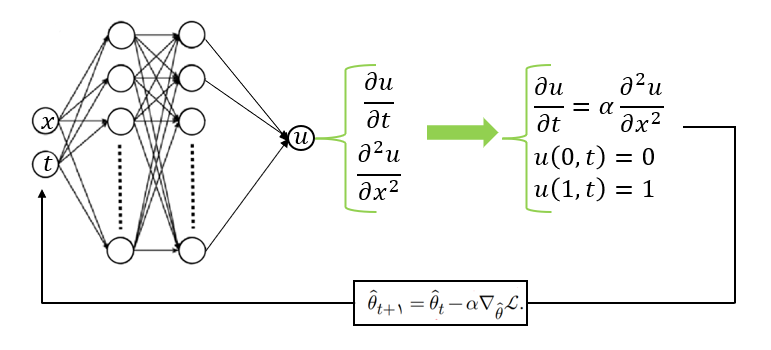
اندازه لایه ورودی: 2
تعداد لایه پنهان: 3
تعداد نورن‌های لایه پنهان: 50
اندازه لایه خروجی: 1
تابع فعال ساز: tanh

فراخوانی کتابخانه‌ها#

تابع `torch.cuda.is_available()` در کتابخانه Pytorch:#

این تابع بررسی می‌کند که آیا سیستم به یک GPU دسترسی دارد یا نه. اگر GPU توسط PyTorch قابل استفاده باشد، مقدار True برمی‌گرداند، در غیر این صورت False.

import torch
import torch.nn as nn
import matplotlib.pyplot as plt
from tqdm import trange
device = 'cuda' if torch.cuda.is_available() else 'cpu'
print(f"Your device is using {device}")

Your device is using cuda

ایجاد داده‌های آموزشی#

تابع torch.meshgrid در PyTorch:#

تابعی است که دو بردار ورودی را گرفته و از آن‌ها شبکه‌ای دوبعدی از مختصات می‌سازد.
indexing ="ij": این دستور به این معنا است که ترتیب ماتریس‌ها به صورت X[i,j]=x[i] و T[i,j]=t[j] است.
indexing="xy": این دستور به این معنا است که ترتیب ماتریس‌ها به صورت X[i,j]=x[j] و T[i,j]=t[i] است.

تابع ravel() در کتابخانه PyTorch:#

این تابع تمامی مقادیر ماتریس X و T را به صورت یک ماتریس تخت یا به صورت یک بردار تبدیل می‌کند.

تابع vstack() در کتابخانه PyTorch:#

این تابع دو تانسور را به صورت عمودی بهم می‌چسباند.

دستور `to(device)` در کتابخانه PyTorch:#

این دستور بسته به مقدار device تانسور‌ها را بر روی CPU یا GPU اجرا می‌کند.

domain = (0, 1)
n_train = 5


x = torch.linspace(domain[0], domain[1], n_train)
t = torch.linspace(domain[0], domain[1], n_train)
x.requires_grad = True
t.requires_grad = True 
# print(x)
# print(t)

X, T = torch.meshgrid((x, t), indexing="ij")
# print(X)
# print(T)
# print(X.ravel())
# print(T.ravel())
points = torch.vstack([X.ravel(), T.ravel()])
# print(points)
points = points.T.to(device)
print(points)

tensor([[0.0000, 0.0000],
        [0.0000, 0.2500],
        [0.0000, 0.5000],
        [0.0000, 0.7500],
        [0.0000, 1.0000],
        [0.2500, 0.0000],
        [0.2500, 0.2500],
        [0.2500, 0.5000],
        [0.2500, 0.7500],
        [0.2500, 1.0000],
        [0.5000, 0.0000],
        [0.5000, 0.2500],
        [0.5000, 0.5000],
        [0.5000, 0.7500],
        [0.5000, 1.0000],
        [0.7500, 0.0000],
        [0.7500, 0.2500],
        [0.7500, 0.5000],
        [0.7500, 0.7500],
        [0.7500, 1.0000],
        [1.0000, 0.0000],
        [1.0000, 0.2500],
        [1.0000, 0.5000],
        [1.0000, 0.7500],
        [1.0000, 1.0000]], device='cuda:0', grad_fn=<ToCopyBackward0>)

ایجاد شبکه عصبی مصنوعی#

torch.manual_seed(42)
class NeuralNet(nn.Module):
    def __init__(self, input_size, hidden_size, output_size):
        super().__init__()
        self.l1 = nn.Linear(input_size, hidden_size)
        self.l2 = nn.Linear(hidden_size, hidden_size)
        self.l3 = nn.Linear(hidden_size, hidden_size)
        self.l4 = nn.Linear(hidden_size, output_size)
        self.tanh = nn.Tanh()
        
    def forward(self, x):
        out = self.tanh(self.l1(x))
        out = self.tanh(self.l2(out))
        out = self.tanh(self.l3(out))
        out = self.l4(out)
        return out
        
input_size, hidden_size, output_size = 2, 50, 1
model = NeuralNet(input_size, hidden_size, output_size)

model.to(device)

NeuralNet(
  (l1): Linear(in_features=2, out_features=50, bias=True)
  (l2): Linear(in_features=50, out_features=50, bias=True)
  (l3): Linear(in_features=50, out_features=50, bias=True)
  (l4): Linear(in_features=50, out_features=1, bias=True)
  (tanh): Tanh()
)

الگوریتم بهینه سازی#

learning_rate = 0.001
optimizer = torch.optim.Adam(model.parameters(), lr=learning_rate)

مشتق‌گیری از خروجی‌های شبکه عصبی#

توضیح درباره خروجی‌های `torch.autograd.grad`#

تابع torch.autograd.grad(outputs, inputs) گرادیان خروجی‌ها را نسبت به ورودی‌ها محاسبه می‌کند و یک لیست از تانسورها باز می‌گرداند. در اینجا، ما از [0] برای دسترسی به اولین (و تنها) عنصر این لیست استفاده می‌کنیم.

۱. وقتی از `[:, 0:1]` و `[:, 1:2]` استفاده می‌کنیم:#

[:, 0:1]: این عبارت مشتق u را نسبت به x (اولین ستون از ورودی‌ها) محاسبه می‌کند.
[:, 1:2]: این عبارت مشتق u را نسبت به t (دومین ستون از ورودی‌ها) محاسبه می‌کند.

۲. وقتی از `[:, :]` استفاده نکنیم:#

اگر از [:, :] یا بدون هیچ ‌زیر مجموعه انتخابی استفاده کنیم، تمام مقادیر گرادیان‌ها (برای هر دو بعد x و t) را به عنوان یک تانسور بدون جدا کردن آن‌ها دریافت خواهیم کرد. به عبارت دیگر، خروجی مشتق دوم شامل تمام مشتقات نسبت به تمام متغیرهای ورودی می‌شود. $$ \frac{\partial^2 u}{\partial (\text{inputs})^2} =

(2)#\[\begin{bmatrix} \displaystyle \frac{\partial}{\partial x}\Bigl(\frac{\partial u}{\partial x} + \frac{\partial u}{\partial t}\Bigr) & \displaystyle \frac{\partial}{\partial t}\Bigl(\frac{\partial u}{\partial x} + \frac{\partial u}{\partial t}\Bigr) \end{bmatrix}\]

=\begin{bmatrix} u_{xx} + u_{tx} & u_{xt} + u_{tt} \end{bmatrix}. $$

def grad(outputs, inputs):
    return torch.autograd.grad(outputs, inputs, grad_outputs=torch.ones_like(outputs), create_graph=True)[0]

# points.requires_grad = True
print(f"inputs: {points}\n")


u = model(points)
print(f"outputs: {u}\n")
dudx = grad(u, points)[:, 0:1]
print(f"the derivative of u with respect to x:{dudx}\n")
d2udx2 = grad(dudx, points)[:, 0:1]
print(f"the second derivative of u with respect to x:{d2udx2}\n")
dudt = grad(u, points)[:, 1:2]
# print(f"the derivative of u with respect to t:{dudt}")

inputs: tensor([[0.0000, 0.0000],
        [0.0000, 0.2500],
        [0.0000, 0.5000],
        [0.0000, 0.7500],
        [0.0000, 1.0000],
        [0.2500, 0.0000],
        [0.2500, 0.2500],
        [0.2500, 0.5000],
        [0.2500, 0.7500],
        [0.2500, 1.0000],
        [0.5000, 0.0000],
        [0.5000, 0.2500],
        [0.5000, 0.5000],
        [0.5000, 0.7500],
        [0.5000, 1.0000],
        [0.7500, 0.0000],
        [0.7500, 0.2500],
        [0.7500, 0.5000],
        [0.7500, 0.7500],
        [0.7500, 1.0000],
        [1.0000, 0.0000],
        [1.0000, 0.2500],
        [1.0000, 0.5000],
        [1.0000, 0.7500],
        [1.0000, 1.0000]], device='cuda:0', grad_fn=<ToCopyBackward0>)

outputs: tensor([[0.0611],
        [0.0672],
        [0.0744],
        [0.0825],
        [0.0913],
        [0.0569],
        [0.0617],
        [0.0678],
        [0.0751],
        [0.0835],
        [0.0546],
        [0.0582],
        [0.0633],
        [0.0698],
        [0.0777],
        [0.0541],
        [0.0568],
        [0.0611],
        [0.0669],
        [0.0742],
        [0.0548],
        [0.0570],
        [0.0608],
        [0.0661],
        [0.0729]], device='cuda:0', grad_fn=<AddmmBackward0>)

the derivative of u with respect to x:tensor([[-0.0205],
        [-0.0258],
        [-0.0301],
        [-0.0331],
        [-0.0346],
        [-0.0129],
        [-0.0181],
        [-0.0225],
        [-0.0257],
        [-0.0275],
        [-0.0053],
        [-0.0095],
        [-0.0133],
        [-0.0163],
        [-0.0184],
        [ 0.0007],
        [-0.0019],
        [-0.0046],
        [-0.0071],
        [-0.0093],
        [ 0.0040],
        [ 0.0030],
        [ 0.0018],
        [ 0.0001],
        [-0.0018]], device='cuda:0', grad_fn=<SliceBackward0>)

the second derivative of u with respect to x:tensor([[0.0279],
        [0.0261],
        [0.0244],
        [0.0231],
        [0.0221],
        [0.0318],
        [0.0339],
        [0.0350],
        [0.0348],
        [0.0335],
        [0.0282],
        [0.0337],
        [0.0374],
        [0.0388],
        [0.0377],
        [0.0189],
        [0.0257],
        [0.0311],
        [0.0340],
        [0.0342],
        [0.0075],
        [0.0135],
        [0.0189],
        [0.0227],
        [0.0245]], device='cuda:0', grad_fn=<SliceBackward0>)

تابع هزینه مسئله معادله گرما#

در این مسئله معادله‌ی زیر را داشتیم:

\[ \frac{\partial u}{\partial t} - 0.4 \frac{\partial^2 u}{\partial x^2} = 0 \]

بخش‌های مختلف تابع هزینه (Loss Terms):#

L_phy: این بخش به معادله دیفرانسیل اصلی مربوط می‌شود

\[ L_{phy} = W_1 \frac{1}{N} \sum_{i=1}^{N} \left(\frac{\partial u_i}{\partial t_i} - 0.4 \frac{\partial^2 u_i}{\partial x_i^2}\right)^2 \]

L_BC1: در شرایط مرزی ( x=0 ) مقدار تابع باید صفر باشد

\[ L_{BC1} = \frac{1}{K} \sum_{i=1}^{K} (u_i(x=0, t_i) - 0)^2 \]

L_BC2 : در شرایط مرزی ( x=1 ) مقدار تابع باید صفر باشد:

\[ L_{BC2} = \frac{1}{K} \sum_{i=1}^{K}(u_i(x=1, t_i) - 0)^2 \]

L_BCs : ترکیب دو شرط مرزی بالا برای نقاط ( x = 0 ) و ( x = 1 ):

\[ L_{BCs} = W_2\frac{1}{(2K)} \sum_{i=1}^{(2K)} u_i(x, t_i)^2 \quad \text{for} \; x=0 \; \& \; x=1 \]

L_IC : شرط اولیه برای زمان ( t = 0 ) به صورت تابع سینوسی زیر است:

\[ L_{IC} = W_3\frac{1}{K} \sum_{i=1}^{K} (u_i(x_i, t=0) - \sin(\pi x_i))^2 \]

🔺 در اینجا باید فقط نقاطی که در آن t = 0 هستند باید انتخاب شوند، یعنی نقاطی مانند (x, t=0) مجاز هستند، ولی نقاطی مانند (x, t=0.1) مجاز نیستند.

✅ نمونه مجاز: (0.5, 0)

❌ نمونه غیر مجاز: (0.5, 1)

تابع نهایی هزینه (Loss):

\[ \text{Loss} = L_{\text{phy}} + L_{\text{BC1}} + L_{\text{BC2}} \]

ایجاد نقاط مرزی#

‍‍points[:, 0] == 0: این دستور تمامی نقاطی را که مقدار x برابر صفر است استخراج میکند. این تابع یک لیست به صورت Boolean بر میگرداند که در آن نقاطی که در شرط مورد نظر صدق می‌کنند True است.
points[:, 0] == 1): این دستور تمامی نقاطی را که مقدار x برابر یک است استخراج میکند. این تابع یک لیست به صورت Boolean بر میگرداند که در آن نقاطی که در شرط مورد نظر صدق می‌کنند True است.
points[:, 1] == 0): این دستور تمامی نقاطی را که مقدار t برابر صفر است استخراج میکند. این تابع یک لیست به صورت Boolean بر میگرداند که در آن نقاطی که در شرط مورد نظر صدق می‌کنند True است.
nonzero(as_tuple=True): این دستور اندیس نقاطی که شرایط برای آنها برقرار است را به صورت tuple بر میگرداند
- خروجی این دستور شامل دو موولفه است که دومین مولفه خالی است و اولین مولفه شامل لیستی از اندیس‌ها است.
‍‍torch.cat([indices1, indices2]): این دستور برای چسباندن دو تانسور به کار می‌رود که اندیس‌های دو مرز را با یکدیگر ترکیب می‌کند تا تمام نقاط مرزی به دست آید.

indices1 = (points[:, 0]==0).nonzero(as_tuple=True)[0]
indices2 = (points[:, 0]==1).nonzero(as_tuple=True)[0]
indices3 = (points[:, 1]==0).nonzero(as_tuple=True)[0]
indices12 = torch.cat([indices1, indices2])
def loss_fn(u, d2udx2, dudt, points, indices12, indices3, weights):
    w1, w2, w3 = weights
    L_phy = w1*torch.mean((dudt - 0.4*d2udx2)**2)
    L_IC = w2*torch.mean((u[indices3] - torch.sin(torch.pi*points[indices3, 0:1]))**2)
    L_BC = w3*torch.mean((u[indices12])**2)
    loss = L_phy + L_BC + L_IC
    return loss, L_phy, L_BC, L_IC

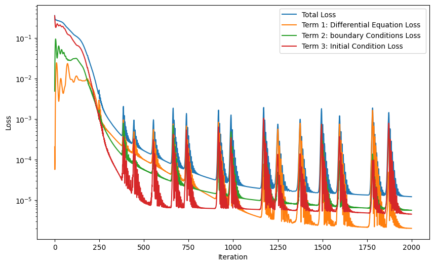
آموزش شبکه عصبی#

num_itrs = 2000
itr_show = 100
weights = (1, 1, 1)

L_total_history = []
L_phy_history = []
L_BC_history = []
L_IC_history = []

pbar = trange(num_itrs)
for itr in pbar:
    u = model(points)
    dudx = grad(u, points)[:, 0:1]
    d2udx2 = grad(dudx, points)[:, 0:1]
    dudt = grad(u, points)[:, 1:2]

    loss, L_phy, L_BC, L_IC = loss_fn(u, d2udx2, dudt, points, indices12, indices3, weights)
    loss.backward()
    optimizer.step()
    optimizer.zero_grad()

    L_total_history.append(loss.item())
    L_phy_history.append(L_phy.item())
    L_BC_history.append(L_BC.item())
    L_IC_history.append(L_IC.item())
    
    pbar.set_postfix({'loss': loss.item()})
    # if itr % itr_show == 0:
    #     print(f'iteration {itr}/{num_itrs}, loss = {loss.item():.6f}')

100%|████████████████████████████████████████████████████████████████| 2000/2000 [00:26<00:00, 74.18it/s, loss=1.21e-5]

بهره‌برداری از شبکه عصبی مصنوعی#

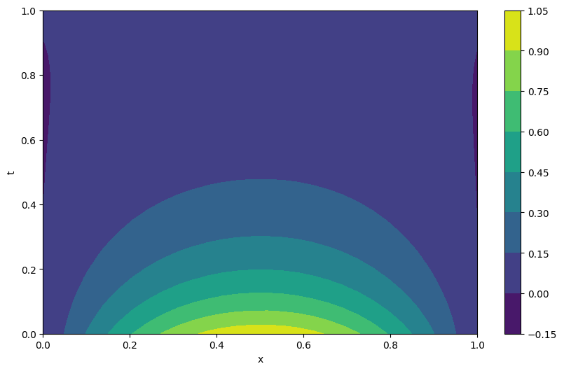
.view(n_test, n_test): از انجایی که داده‌های خروجی در قالب یک بردار یک بعدی هستند برای رسم دو بعدی باید به شکل (n_test, n_test) بازآرایی کرد. اینکار باعث می‌شود داده‌های در شبکه‌ای مقادیر x و t قابل ترسیم باشند.
plt.contourf(): ما تابع مدل را در صفحه‌ی (x, t) محاسبه کرده‌ایم. با استفاده از plt.contourf می‌توانیم توزیع این تابع را در زمان‌ها و مکان‌های مختلف ببینیم.

n_test = 30
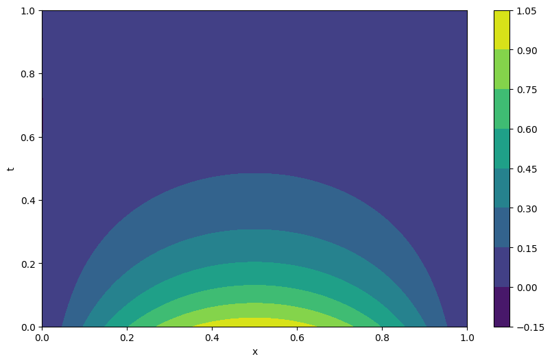
def exact_solution(points):
    x, t = points[:, 0:1], points[:, 1:2]
    return torch.exp(-0.4*(torch.pi**2)*t) * torch.sin(torch.pi*x)
    
t = torch.linspace(domain[0], domain[1], n_test)
x = torch.linspace(domain[0], domain[1], n_test)

X, T = torch.meshgrid((x, t), indexing="ij")
points = torch.vstack([X.ravel(), T.ravel()]).T.to(device)


predicted = model(points)

analytic_cal = exact_solution(points)

mse = torch.mean((predicted - analytic_cal)**2)
print(f"MSE error: {mse}")

predicted = predicted.view(n_test, n_test)
analytic_cal = analytic_cal.view(n_test, n_test)

plt.figure(figsize=(10, 6))
cp = plt.contourf(X.detach().numpy(), T.detach().numpy(), predicted.cpu().detach().numpy())
plt.colorbar(cp)
plt.xlabel('x')
plt.ylabel('t')
plt.show()

plt.figure(figsize=(10, 6))
cp = plt.contourf(X.detach().numpy(), T.detach().numpy(), analytic_cal.cpu().detach().numpy())
plt.colorbar(cp)
plt.xlabel('x')
plt.ylabel('t')
plt.show()

plt.figure(figsize=(10, 6))
plt.semilogy(L_total_history, label="Total Loss")
plt.semilogy(L_phy_history, label="Term 1: Differential Equation Loss")
plt.semilogy(L_BC_history, label="Term 2: boundary Conditions Loss ")
plt.semilogy(L_IC_history, label="Term 3: Initial Condition Loss")
plt.xlabel('Iteration')
plt.ylabel('Loss')
plt.legend()
plt.show()

MSE error: 1.2524047633633018e-05

../_images/cadf36f0115bdc3f0895b100fc9d8b5cf70e1ea149212dd80a6fac34af467de9.png

../_images/49cdbb8c6d15913617b1876c4bef926610bfe21b478d996e37c7f7c658ebeb9a.png

../_images/892d42e646845d5714d407a8b7e758c7254f0acc31c3f8941ac98355a2e9d0db.png

پیاده‌سازی نهایی#

import torch
import torch.nn as nn
import matplotlib.pyplot as plt
from tqdm import trange
device = 'cuda' if torch.cuda.is_available() else 'cpu'
print(f"Your device is using {device}")

class NeuralNet(nn.Module):
    def __init__(self, input_size, hidden_size, output_size):
        super().__init__()
        self.l1 = nn.Linear(input_size, hidden_size)
        self.l2 = nn.Linear(hidden_size, hidden_size)
        self.l3 = nn.Linear(hidden_size, hidden_size)
        self.l4 = nn.Linear(hidden_size, output_size)
        self.tanh = nn.Tanh()
        
    def forward(self, x):
        out = self.tanh(self.l1(x))
        out = self.tanh(self.l2(out))
        out = self.tanh(self.l3(out))
        out = self.l4(out)
        return out


class Trainer:
    def __init__(self, model, optimizer, domain, weights):
        self.model = model
        self.optimizer = optimizer
        self.domain = domain
        self.weights = weights

        self.L_total_history = []
        self.L_phy_history = []
        self.L_BC_history = []
        self.L_IC_history = []

    def exact_solution(self, points):
        x, t = points[:, 0:1], points[:, 1:2]
        return torch.exp(-0.4*(torch.pi**2)*t) * torch.sin(torch.pi*x)

    def grad(self, outputs, inputs):
        return torch.autograd.grad(outputs, inputs, grad_outputs=torch.ones_like(outputs), create_graph=True)[0]

    def generate_data(self, n_data):
        t = torch.linspace(self.domain[0], self.domain[1], n_data)
        x = torch.linspace(self.domain[0], self.domain[1], n_data)
        
        X, T = torch.meshgrid((x, t), indexing="ij")
        data = torch.vstack([X.ravel(), T.ravel()]).T.to(device)
        
        return X, T, data

    def loss_fn(self, u, d2udx2, dudt, points, indices12, indices3, weights):
        w1, w2, w3 = weights
        L_phy = w1*torch.mean((dudt - 0.4*d2udx2)**2)
        L_IC = w2*torch.mean((u[indices3] - torch.sin(torch.pi*points[indices3, 0:1]))**2)
        L_BC = w3*torch.mean((u[indices12])**2)
        loss = L_phy + L_BC + L_IC
        return loss, L_phy, L_BC, L_IC

    def train(self, n_train, num_itr, show_itr=False):

        
        X, T, points = self.generate_data(n_train)
        points.requires_grad = True


        indices1 = (points[:, 0]==0).nonzero(as_tuple=True)[0]
        indices2 = (points[:, 0]==1).nonzero(as_tuple=True)[0]
        indices3 = (points[:, 1]==0).nonzero(as_tuple=True)[0]
        indices12 = torch.cat([indices1, indices2])

        
        pbar = trange(num_itr)
        for itr in pbar:
            u = model(points)
            dudx = self.grad(u, points)[:, 0:1]
            d2udx2 = self.grad(dudx, points)[:, 0:1]
            dudt = self.grad(u, points)[:, 1:2]
        
            loss, L_phy, L_BC, L_IC = self.loss_fn(u, d2udx2, dudt, points, indices12, indices3, weights)
            loss.backward()
            optimizer.step()
            optimizer.zero_grad()
        
            self.L_total_history.append(loss.item())
            self.L_phy_history.append(L_phy.item())
            self.L_BC_history.append(L_BC.item())
            self.L_IC_history.append(L_IC.item())
        
            
            if show_itr and itr % 100 == 0:
                print(f'iteration {itr}/{num_itr}, loss = {loss.item():.6f}')
            else:
                pbar.set_postfix({'loss': loss.item()})


    def evaluation(self, n_test):
        X, T, points = self.generate_data(n_test)

        predicted = self.model(points)
        
        analytic_cal = self.exact_solution(points)
        
        mse = torch.mean((predicted - analytic_cal)**2)
        print(f"MSE error: {mse}")
        
        predicted = predicted.view(n_test, n_test)
        analytic_cal = analytic_cal.view(n_test, n_test)
        
        plt.figure(figsize=(10, 6))
        cp = plt.contourf(X.detach().numpy(), T.detach().numpy(), predicted.cpu().detach().numpy())
        plt.colorbar(cp)
        plt.xlabel('x')
        plt.ylabel('t')
        plt.show()
        
        plt.figure(figsize=(10, 6))
        cp = plt.contourf(X.detach().numpy(), T.detach().numpy(), analytic_cal.cpu().detach().numpy())
        plt.colorbar(cp)
        plt.xlabel('x')
        plt.ylabel('t')
        plt.show()
        
        plt.figure(figsize=(10, 6))
        plt.semilogy(self.L_total_history, label="Total Loss")
        plt.semilogy(self.L_phy_history, label="Term 1: Differential Equation Loss")
        plt.semilogy(self.L_BC_history, label="Term 2: boundary Conditions Loss")
        plt.semilogy(self.L_IC_history, label="Term 3: Initial Condition Loss")
        plt.xlabel('Iteration')
        plt.ylabel('Loss')
        plt.legend()
        plt.show()

Your device is using cuda

torch.manual_seed(42)
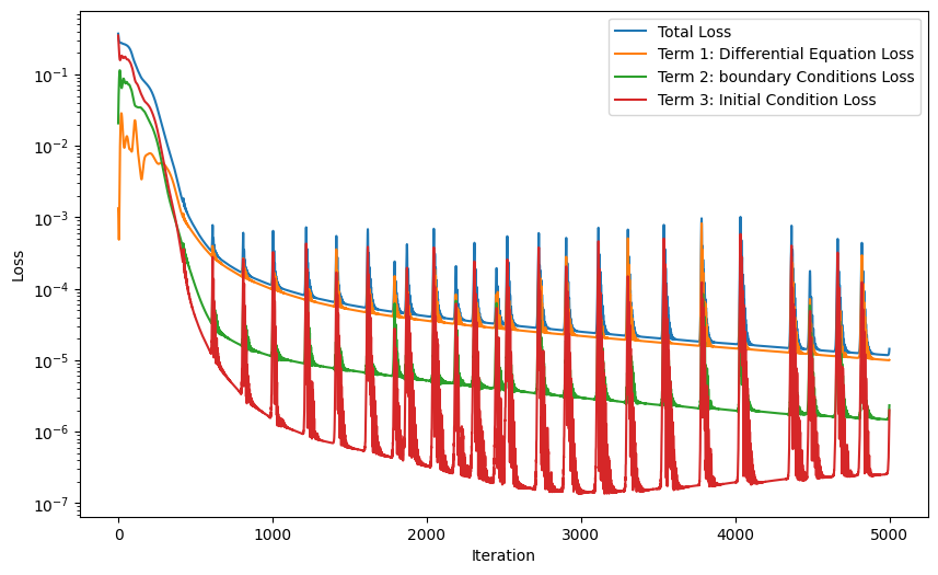
n_train, n_test, num_itr, itr_show = 30, 100, 5000, 1000
weights, domain = (1, 1, 1), (0, 1)
learning_rate = 0.001
input_size, hidden_size, output_size = 2, 30, 1

model = NeuralNet(input_size, hidden_size, output_size).to(device)
optimizer = torch.optim.Adam(model.parameters(), lr=learning_rate)

trainer = Trainer(model, optimizer, domain, weights)

trainer.train(n_train, num_itr, show_itr=False)

trainer.evaluation(n_test)

100%|████████████████████████████████████████████████████████████████| 5000/5000 [01:02<00:00, 80.62it/s, loss=1.44e-5]

MSE error: 2.189112137784832e-06

../_images/e4355a8a950ecd5800cac5d99d354d817558e45877f66df539a5b5a4f53ca0f0.png

../_images/d5e798971ac4616bf9af95ad72112b6295121985f8adf92f5b34ab1d45b0ae1e.png

../_images/bc760a2ceb4731df6eb6a5b4a611b6ee39c5a32f729b45567710e72e4a98f78a.png

معادله لاپلاس بر روی یک دیسک#

حل معادله لاپلاس در ناحیه‌ای به شکل دیسک واحد با استفاده از شبکه‌های عصبی:

\[ r \frac{\partial u}{\partial r} + r^2 \frac{\partial^2 u}{\partial r^2} + \frac{\partial^2 u}{\partial \theta^2} = 0 \]

شناخت مسئله#

1. شرط مرزی اول#

مقدار تابع $u$ روی مرز دیسک (برای $r=1$) به صورت زیر داده شده است:

\[ u(1, \theta) = \cos(\theta) \]

2. شرط مرزی دوم#

\[ u(r, \theta + 2\pi) = u(r, \theta) \]

3. حل تحلیلی#

حل تحلیلی معادله لاپلاس برای این شرایط مرزی در دستگاه مختصات قطبی به صورت زیر است:

\[ u(r, \theta) = r \cos(\theta) \]

4. مشخصات ساختار شبکه عصبی مصنوعی#

Alt Text

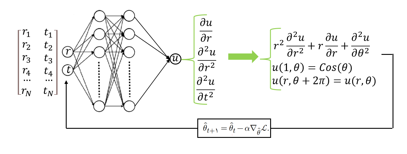
اندازه لایه ورودی: 2 (مختصات $r$ و $\theta$)
تعداد لایه پنهان: ۳
تعداد نورون‌های لایه پنهان: ۵۰
اندازه لایه خروجی: ۱
تابع فعال‌ساز: $\tanh$

فراخوانی کتابخانه‌ها#

import torch
import torch.nn as nn
import matplotlib.pyplot as plt
from tqdm import trange
device = 'cuda' if torch.cuda.is_available() else 'cpu'
print(f"Your device is using {device}")

Your device is using cuda

ایجاد داده‌های آموزشی برای آموزش شبکه عصبی مصنوعی#

domain1 = (0, 2*torch.pi) # theta
domain2 = (0, 1) # r
n_train = 30
t = torch.linspace(domain1[0], domain1[1], n_train)
r = torch.linspace(domain2[0], domain2[1], n_train)
R, T = torch.meshgrid((r, t), indexing="ij")
points = torch.vstack([R.ravel(), T.ravel()]).T.to(device)

ایجاد شبکه عصبی و الگوریتم بهینه‌سازی#

torch.manual_seed(42)

class NeuralNet(nn.Module):
    def __init__(self, input_size, hidden_size, output_size):
        super().__init__()
        self.l1 = nn.Linear(input_size, hidden_size)
        self.l2 = nn.Linear(hidden_size, hidden_size)
        self.l3 = nn.Linear(hidden_size, hidden_size)
        self.l4 = nn.Linear(hidden_size, output_size)
        self.tanh = nn.Tanh()
        
    def forward(self, x):
        out = self.tanh(self.l1(x))
        out = self.tanh(self.l2(out))
        out = self.tanh(self.l3(out))
        out = self.l4(out)
        return out
        
input_size, hidden_size, output_size = 2, 50, 1
model = NeuralNet(input_size, hidden_size, output_size).to(device)

learning_rate = 0.001
optimizer = torch.optim.Adam(model.parameters(), lr=learning_rate)

مشتق‌گیری از خروجی‌های شبکه عصبی#

def grad(outputs, inputs):
    return torch.autograd.grad(outputs, inputs, grad_outputs=torch.ones_like(outputs), create_graph=True)[0]
    
points.requires_grad = True
u = model(points)

dudr = grad(u, points)[:, 0:1]
d2udr2 = grad(dudr, points)[:, 0:1]
dudt = grad(u, points)[:, 1:2]
d2udt2 = grad(dudt, points)[:, 1:2]

تابع هزینه برای حل معادله لاپلاس بر روی یک دیسک (در مختصات قطبی)#

در این مسئله، معادله‌ی لاپلاس در مختصات قطبی به صورت زیر داده شده است:

\[ r \frac{\partial u}{\partial r} + r^2 \frac{\partial^2 u}{\partial r^2} + \frac{\partial^2 u}{\partial \theta^2} = 0 \]

بخش‌های مختلف تابع هزینه (Loss Terms):#

L_phy: این بخش به معادله دیفرانسیل اصلی مربوط می‌شود

\[ L_{\text{phy}} = W_1 \cdot \frac{1}{N} \sum_{i=1}^{N} \left( r_i \cdot \frac{\partial u_i}{\partial r_i} + r_i^2 \cdot \frac{\partial^2 u_i}{\partial r_i^2} + \frac{\partial^2 u_i}{\partial \theta_i^2} \right)^2 \]

L_BC1: در شرایط مرزی مقادیر تابع در (r=1) باید برابر $cos(\theta)$ باشد:

\[ L_{\text{BC1}} = W_2 \cdot \frac{1}{K} \sum_{i=1}^{K} \left(u_i(r=1, \theta_i) - \cos(\theta_i)\right)^2 \]

L_BC2: در شرایط مرزی دوره‌ای مقادیر تابع برای نقاطی که در آنها $\theta=0$ و $\theta=2\pi$ است باید با یکدیگر برابر باشد

\[ L_{\text{BC2}} = W_3 \cdot \frac{1}{K} \sum_{i=1}^{K} \left(u_i(r_i, \theta=2\pi) - u_i(r_i, \theta=0)\right)^2 \]

تابع نهایی هزینه (Loss):

\[ \text{Loss} = L_{\text{phy}} + L_{\text{BC1}} + L_{\text{BC2}} \]

indices1 = (points[:, 0]==1).nonzero(as_tuple=True)[0].to(device)
indices2 = (points[:, 1]==2*torch.pi).nonzero(as_tuple=True)[0].to(device)
indices3 = (points[:, 1]==0).nonzero(as_tuple=True)[0].to(device)

def loss_fn(u, dudr, d2udr2, d2udt2, points, indices1, indices2, indices3, weights):
    w1, w2, w3 = weights

    L_phy = w1*torch.mean((points[:, 0:1]*dudr + (points[:, 0:1]**2)*d2udr2 + d2udt2)**2)
    L_BC1 = w2*torch.mean((u[indices1] - torch.cos(points[indices1, 1:2]))**2)
    L_BC2 = w3*torch.mean((u[indices2] - u[indices3])**2)
    loss = L_phy + L_BC1 + L_BC2
    
    return loss, L_phy, L_BC1, L_BC2

آموزش شبکه عصبی#

num_itrs = 2000
itr_show = 100
weights = (1, 1, 1)



L_total_history = []
L_phy_history = []
L_BC1_history = []
L_BC2_history = []

pbar = trange(num_itrs)
for itr in pbar:
    u = model(points)
    
    dudr = grad(u, points)[:, 0:1]
    d2udr2 = grad(dudr, points)[:, 0:1]
    dudt = grad(u, points)[:, 1:2]
    d2udt2 = grad(dudt, points)[:, 1:2]
    
    loss, L_phy, L_BC1, L_BC2 = loss_fn(u, dudr, d2udr2, d2udt2, points, indices1, indices2, indices3, weights)
    loss.backward()
    optimizer.step()
    optimizer.zero_grad()

    L_total_history.append(loss.item())
    L_phy_history.append(L_phy.item())
    L_BC1_history.append(L_BC1.item())
    L_BC2_history.append(L_BC2.item())
    
    pbar.set_postfix({'loss': loss.item()})
    # if itr % itr_show == 0:
    #     print(f'iteration {itr}/{num_itrs}, loss = {loss.item():.6f}')

100%|█████████████████████████████████████████████████████████████████| 2000/2000 [00:33<00:00, 59.82it/s, loss=0.0012]

بهره‌برداری از شبکه عصبی مصنوعی#

n_test = 50

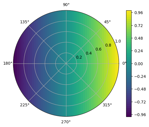
def exact_solution(points):
    r, t = points[:, 0:1], points[:, 1:2]
    return r*torch.cos(t)

t = torch.linspace(domain1[0], domain1[1], n_test)
r = torch.linspace(domain2[0], domain2[1], n_test)
R, T = torch.meshgrid((r, t), indexing="ij")
data = torch.vstack([R.ravel(), T.ravel()]).T


predicted = model(data.to(device))
analytic_cal = exact_solution(data).to(device)

mse = torch.mean((predicted - analytic_cal)**2)
print(f"MSE error: {mse}")

predicted = predicted.view(n_test, n_test)
analytic_cal = analytic_cal.view(n_test, n_test)

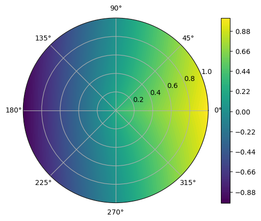
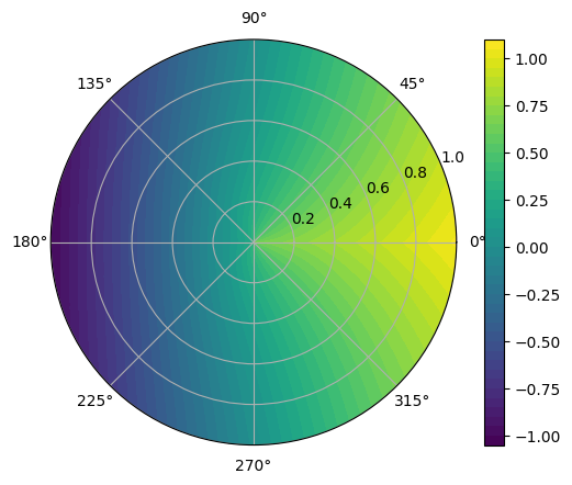
fig = plt.figure()
ax = fig.add_subplot(111, polar=True)
c = ax.contourf(T.detach().numpy(), R.detach().numpy(), predicted.cpu().detach().numpy(), 50, cmap='viridis')
fig.colorbar(c)
plt.show()

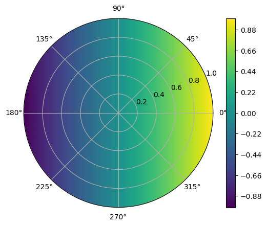
fig = plt.figure()
ax = fig.add_subplot(111, polar=True)
c = ax.contourf(T.detach().numpy(), R.detach().numpy(), analytic_cal.cpu().detach().numpy(), 50, cmap='viridis')
fig.colorbar(c)
plt.show()

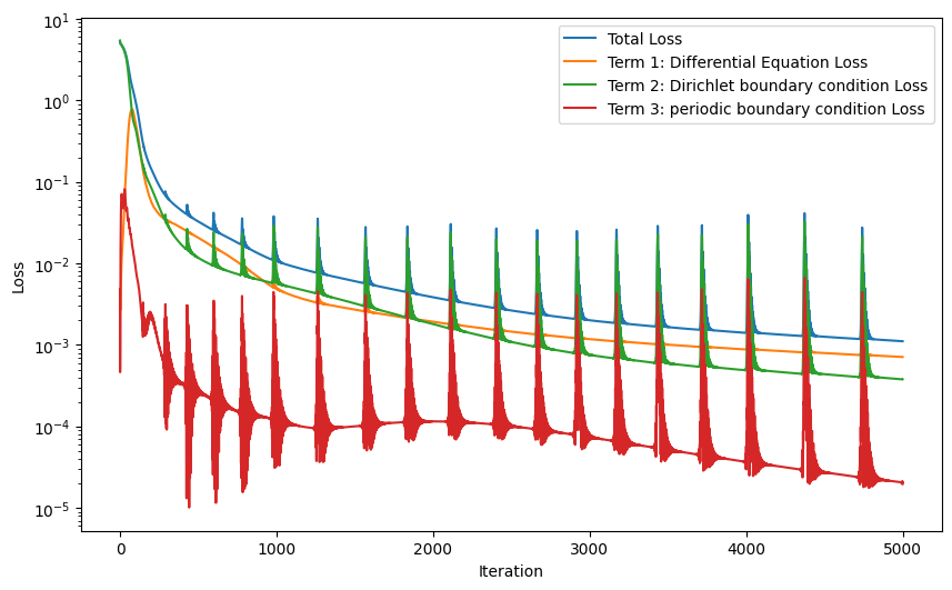
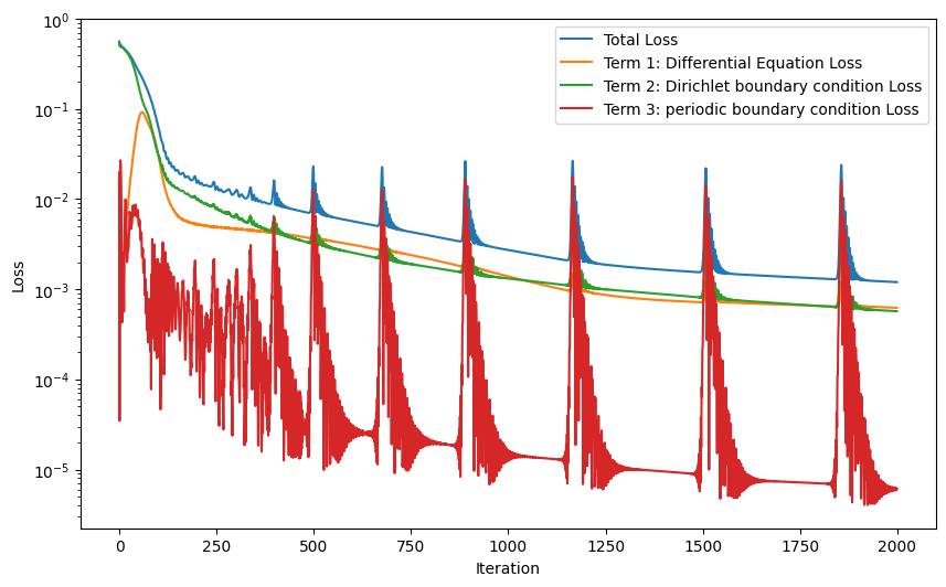
plt.figure(figsize=(10, 6))
plt.semilogy(L_total_history, label="Total Loss")
plt.semilogy(L_phy_history, label="Term 1: Differential Equation Loss")
plt.semilogy(L_BC1_history, label="Term 2: Dirichlet boundary condition Loss")
plt.semilogy(L_BC2_history, label="Term 3: periodic boundary condition Loss")
plt.xlabel('Iteration')
plt.ylabel('Loss')
plt.legend()
plt.show()

MSE error: 0.0494583323597908

../_images/4d09e65f8a5087a81e1497ac53405151724ff497ad3453cc1d8504e3774e6188.png

../_images/8c4108d305b80fa2fc90352a2e07d884c7db9357da4dea1b73a114b87b98c5b9.png

../_images/f666b3c0d387b312f0bf5b3be5def3c05af1e577f416bb115fdc2dfed1c7a3ff.png

پیاده‌سازی نهایی#

import torch
import torch.nn as nn
import matplotlib.pyplot as plt
from tqdm import trange
device = 'cuda' if torch.cuda.is_available() else 'cpu'
print(f"Your device is using {device}")

class NeuralNet(nn.Module):
    def __init__(self, input_size, hidden_size, output_size):
        super().__init__()
        self.l1 = nn.Linear(input_size, hidden_size)
        self.l2 = nn.Linear(hidden_size, hidden_size)
        self.l3 = nn.Linear(hidden_size, hidden_size)
        self.l4 = nn.Linear(hidden_size, output_size)
        self.tanh = nn.Tanh()
        
    def forward(self, x):
        out = self.tanh(self.l1(x))
        out = self.tanh(self.l2(out))
        out = self.tanh(self.l3(out))
        out = self.l4(out)
        return out


class Trainer:
    def __init__(self, model, optimizer, domain1, domain2, weights):
        self.model = model
        self.optimizer = optimizer
        self.domain1 = domain1
        self.domain2 = domain2
        self.weights = weights

        self.L_total_history = []
        self.L_phy_history = []
        self.L_BC1_history = []
        self.L_BC2_history = []

    def exact_solution(self, points):
        r, t = points[:, 0:1], points[:, 1:2]
        return r*torch.cos(t)

    def grad(self, outputs, inputs):
        return torch.autograd.grad(outputs, inputs, grad_outputs=torch.ones_like(outputs), create_graph=True)[0]

    def generate_data(self, n_data):
        t = torch.linspace(self.domain1[0], self.domain1[1], n_data)
        r = torch.linspace(self.domain2[0], self.domain2[1], n_data)
        R, T = torch.meshgrid((r, t), indexing="ij")
        data = torch.vstack([R.ravel(), T.ravel()]).T.to(device)
        return R, T, data

    def loss_fn(self, u, dudr, d2udr2, d2udt2, points, indices1, indices2, indices3, weights):
        w1, w2, w3 = weights
        L_phy = w1*torch.mean((points[:, 0:1]*dudr + (points[:, 0:1]**2)*d2udr2 + d2udt2)**2)
        L_BC1 = w2*torch.mean((u[indices1] - torch.cos(points[indices1, 1:2]))**2)
        L_BC2 = w3*torch.mean((u[indices2] - u[indices3])**2)
        loss = L_phy + L_BC1 + L_BC2
        return loss, L_phy, L_BC1, L_BC2

    def train(self, n_train, num_itr, show_itr=False):

        
        R, T, points = self.generate_data(n_train)
        points.requires_grad = True


        indices1 = (points[:, 0]==1).nonzero(as_tuple=True)[0].to(device)
        indices2 = (points[:, 1]==2*torch.pi).nonzero(as_tuple=True)[0].to(device)
        indices3 = (points[:, 1]==0).nonzero(as_tuple=True)[0].to(device)

        pbar = trange(num_itr)
        for itr in pbar:
            u = self.model(points)

            dudr = self.grad(u, points)[:, 0:1]
            d2udr2 = self.grad(dudr, points)[:, 0:1]
            dudt = self.grad(u, points)[:, 1:2]
            d2udt2 = self.grad(dudt, points)[:, 1:2]
            
            loss, L_phy, L_BC1, L_BC2 = self.loss_fn(u, dudr, d2udr2, d2udt2, points, indices1, indices2, indices3, weights)
            loss.backward()
            optimizer.step()
            optimizer.zero_grad()
        
            self.L_total_history.append(loss.item())
            self.L_phy_history.append(L_phy.item())
            self.L_BC1_history.append(L_BC1.item())
            self.L_BC2_history.append(L_BC2.item())
        

            if show_itr and itr % 100 == 0:
                print(f'iteration {itr}/{num_itr}, loss = {loss.item():.6f}')
            else:
                pbar.set_postfix({'loss': loss.item()})


    def evaluation(self, n_test):
        R, T, points = self.generate_data(n_test)
        predicted = self.model(points.to(device))
        analytic_cal = self.exact_solution(points).to(device)
        
        mse = torch.mean((predicted - analytic_cal)**2)
        print(f"MSE error: {mse}")

        predicted = predicted.view(n_test, n_test)
        analytic_cal = analytic_cal.view(n_test, n_test)
        
        fig = plt.figure()
        ax = fig.add_subplot(111, polar=True)
        c = ax.contourf(T.detach().numpy(), R.detach().numpy(), predicted.cpu().detach().numpy(), 100,cmap='viridis')
        fig.colorbar(c)
        plt.show()
        
        fig = plt.figure()
        ax = fig.add_subplot(111, polar=True)
        c = ax.contourf(T.detach().numpy(), R.detach().numpy(), analytic_cal.cpu().detach().numpy(), 100,cmap='viridis')
        fig.colorbar(c)
        plt.show()
        
        plt.figure(figsize=(10, 6))
        plt.semilogy(self.L_total_history, label="Total Loss")
        plt.semilogy(self.L_phy_history, label="Term 1: Differential Equation Loss")
        plt.semilogy(self.L_BC1_history, label="Term 2: Dirichlet boundary condition Loss")
        plt.semilogy(self.L_BC2_history, label="Term 3: periodic boundary condition Loss")
        plt.xlabel('Iteration')
        plt.ylabel('Loss')
        plt.legend()
        plt.show()

Your device is using cuda

torch.manual_seed(42)
n_train, n_test, num_itr, itr_show = 30, 100, 5000, 1000
weights, domain1, domain2 = (5, 10, 1), (0, 2*torch.pi), (0, 1)
learning_rate = 0.001
input_size, hidden_size, output_size = 2, 30, 1

model = NeuralNet(input_size, hidden_size, output_size).to(device)
optimizer = torch.optim.Adam(model.parameters(), lr=learning_rate)

trainer = Trainer(model, optimizer, domain1, domain2, weights)

trainer.train(n_train, num_itr, show_itr=False)

trainer.evaluation(n_test)

100%|████████████████████████████████████████████████████████████████| 5000/5000 [01:15<00:00, 65.93it/s, loss=0.00111]

MSE error: 0.01583779789507389

../_images/b7cd4782d29cfcdfd25694f51a5e707492caec606ffeffff550f71ecb290bd5d.png

../_images/403a3ba255f222665bac3a990601026fced033df6a77cefe6a8d5ea1658502a0.png

../_images/b59db53e32d730fc9d31d415d8ca24aa3240c7f6590a538d44f51813be41f1ed.png

حل چند معادله دیفرانسیل

Contents

حل چند معادله دیفرانسیل#

Heat Equation (معادله گرمایی)#

1. Boundary Conditions (شرایط مرزی)#

2. Initial Condition (شرط اولیه)#

3. Analytical Solution (حل تحلیلی)#

مشخصات ساختار شبکه عصبی مصنوعی#

فراخوانی کتابخانه‌ها#

تابع torch.cuda.is_available() در کتابخانه Pytorch:#

ایجاد داده‌های آموزشی#

تابع torch.meshgrid در PyTorch:#

تابع ravel() در کتابخانه PyTorch:#

تابع vstack() در کتابخانه PyTorch:#

دستور to(device) در کتابخانه PyTorch:#

ایجاد شبکه عصبی مصنوعی#

الگوریتم بهینه سازی#

مشتق‌گیری از خروجی‌های شبکه عصبی#

توضیح درباره خروجی‌های torch.autograd.grad#

۱. وقتی از [:, 0:1] و [:, 1:2] استفاده می‌کنیم:#

۲. وقتی از [:, :] استفاده نکنیم:#

تابع هزینه مسئله معادله گرما#

بخش‌های مختلف تابع هزینه (Loss Terms):#

ایجاد نقاط مرزی#

آموزش شبکه عصبی#

بهره‌برداری از شبکه عصبی مصنوعی#

پیاده‌سازی نهایی#

معادله لاپلاس بر روی یک دیسک#

شناخت مسئله#

1. شرط مرزی اول#

2. شرط مرزی دوم#

3. حل تحلیلی#

4. مشخصات ساختار شبکه عصبی مصنوعی#

فراخوانی کتابخانه‌ها#

ایجاد داده‌های آموزشی برای آموزش شبکه عصبی مصنوعی#

ایجاد شبکه عصبی و الگوریتم بهینه‌سازی#

مشتق‌گیری از خروجی‌های شبکه عصبی#

تابع هزینه برای حل معادله لاپلاس بر روی یک دیسک (در مختصات قطبی)#

بخش‌های مختلف تابع هزینه (Loss Terms):#

آموزش شبکه عصبی#

بهره‌برداری از شبکه عصبی مصنوعی#

پیاده‌سازی نهایی#

تابع `torch.cuda.is_available()` در کتابخانه Pytorch:#

دستور `to(device)` در کتابخانه PyTorch:#

توضیح درباره خروجی‌های `torch.autograd.grad`#

۱. وقتی از `[:, 0:1]` و `[:, 1:2]` استفاده می‌کنیم:#

۲. وقتی از `[:, :]` استفاده نکنیم:#